Exploratory Data Analysis of Housing Rental Market in Germany with Python

Data Collection

For data collection, we use ImmoScout24, one of the vast and oldest websites comprising more than 72,000 apartments and houses. The website has an API and a page for developers. However, we will scrape real estate data using Python.

Before data collection, ensure to seek permission from the owner. Never use several threads at a time. It will prevent the server from overloading. For debugging your code, use the saved HTML files.

For exploratory data analysis with Python, first, we will get the page data using requests.

But we need something else because the page has protection against robots. Hence, the Selenium Python library uses a real Chrome browser to save the data and automate the reading pages.

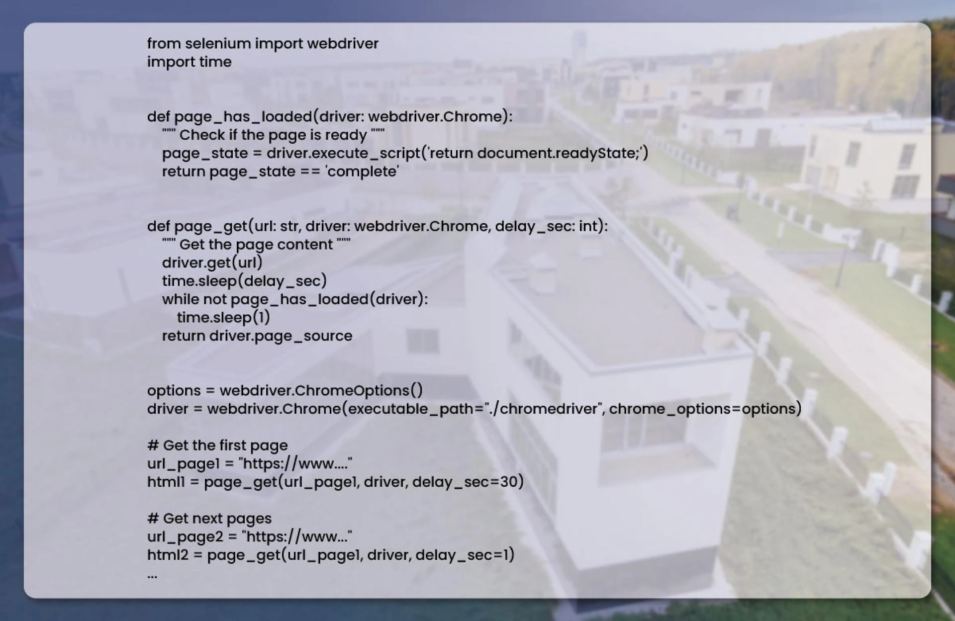
As soon as the code runs, the browser window gets open. Before processing the first page, we added a 30-second delay to ensure that we were not a robot. Within this interval, press the three dots at the right to open the browser setting and disable the loading of images.

The browser gets opened up during requests for the following pages, and there is no robot check for further data. After getting the HTML body, the data extraction of housing rental becomes easy. Use the Inspect button to find the HTML element properties.

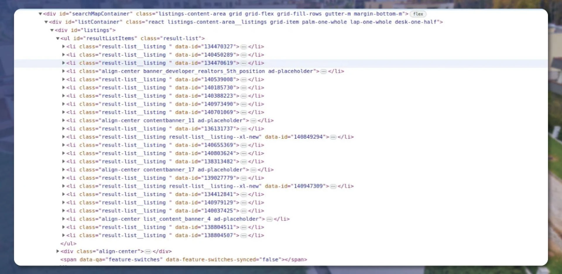
We will get these elements in Python using the BeautifulSoup library. The code will extract all the apartment URLs from the page.

Let’s find the type of data we need.

Data Fields

For each estate object, we will have a page like this. The value and name of the company are a blur.

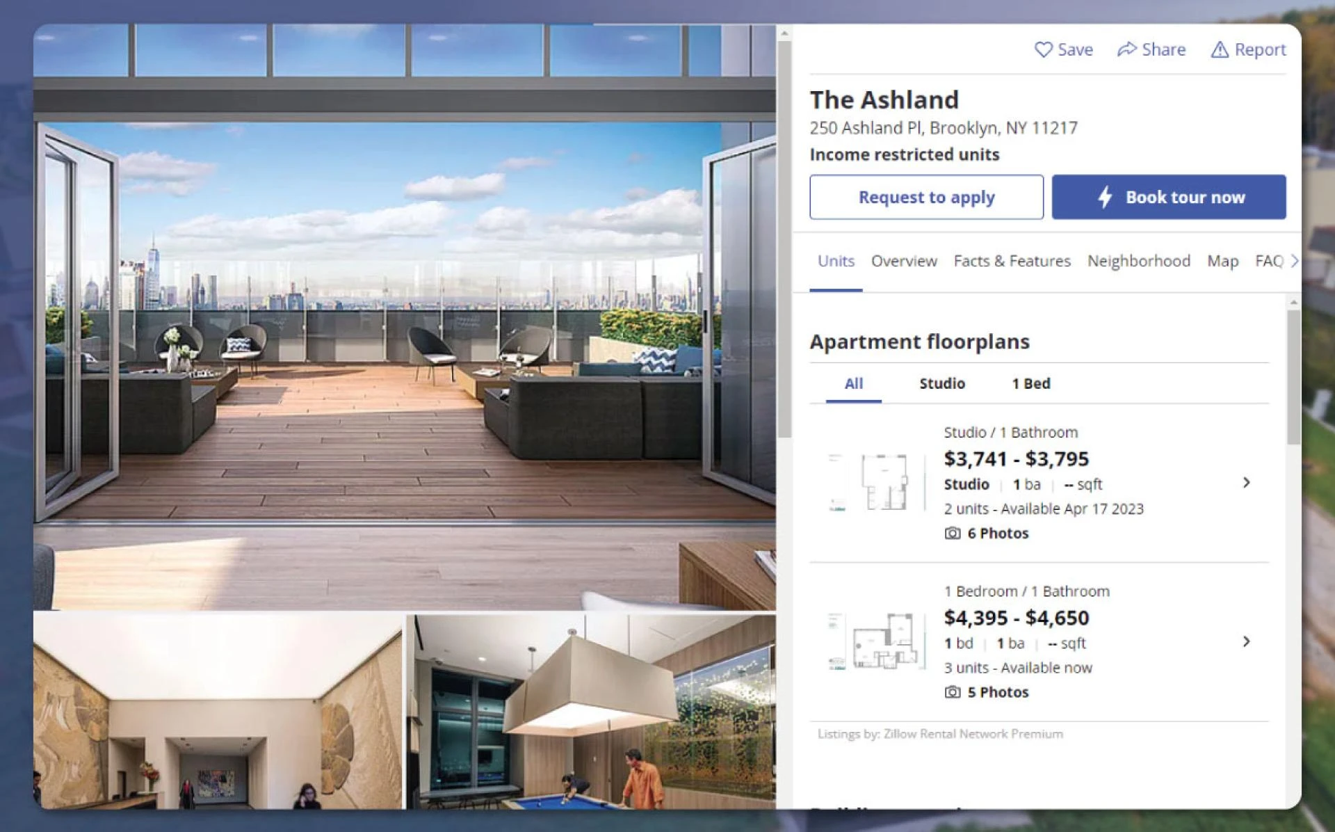
Below are the types of data we can get:

Title : In the above picture is a single apartment in Hermsdorf. But, this text needs to be more helpful for data analysis.

Type : The type is Etagenwohnung (apartment situated on the floor).

Kaltmiete or cold price : includes the rental price except the utility costs, like electricity or heating.

Warmmiete or warm price : Apart from heating costs, it includes certain other costs.

Etage or floor : On this page lies text 0-3. Hence a tiny parsing is needed. In Germany, the first floor is considered the first elevated. Hence, we will consider 0 as the ground floor in German. From 0 to 3, we can extract the total number of floors in the building.

Kaution (deposit) : Here, we will find a value of 3-Kalmieten. Specific parsing is

Flasche (area) : It includes the house or apartment area.

Zimmer (room) : It is 1.

You can also extract several other data fields, like, extra rent for a garage, pet allowances, etc. As we performed earlier, the process of HTML parsing is precisely the same. To obtain the property title, we will use the below code.

Similarly, we find for other fields. After running the code for all pages, we will obtain the datasets like this and save them in a CSV format.

Let’s see what information we can avail.

Data Cleaning & Transformation

The housing data will require cleaning and transformation to obtain a structured format.

We have collected the data from 6 cities in different parts of Germany. It includes Berlin, Frankfurt, Munchen, Koln, Hamburg, and Dresden. We will check for Berlin. We will first load the CSV into the Panda data frame.

At first, the let’s do parsing using Python, and for all missing values, “None” was written in the CSV. As we don’t require None, we specify it as ‘na_values.’ For the separator, we used “.” And set ‘pd.INT32Dtype’ for integer fields, including floor number and price. The output will look like this:

We will then check for dimensionality and the number of NULL values.

The output will appear like this:

The above image shows that the total number of properties in Berlin is 3556. Each property has cold and warm prices, number of rooms, area, etc. For 2467 properties, a ‘type’ is missing. There needs to be a floor value for 2200 properties, and so on. Hence, we will require a method to convert test strings like ‘3 Nettokalmieten’ to numeric values.

Basic Analysis

We will use the Pandas method ‘describe’ to get descriptive statistics of the dataset.

We removed the ‘property id’ from the results and adjusted the output by adding a ‘thousand’ separator. The Berlin results will appear like this.

From the above image, we can see that 3556 properties are available in Berlin. The 50th percentile area for those 3,556 properties is 60 square meters. Its median price is € 1,645. The 75th percentile is €2,271. It indicates that 75% of the property value is cheaper than this value. The average number of rooms is 2.

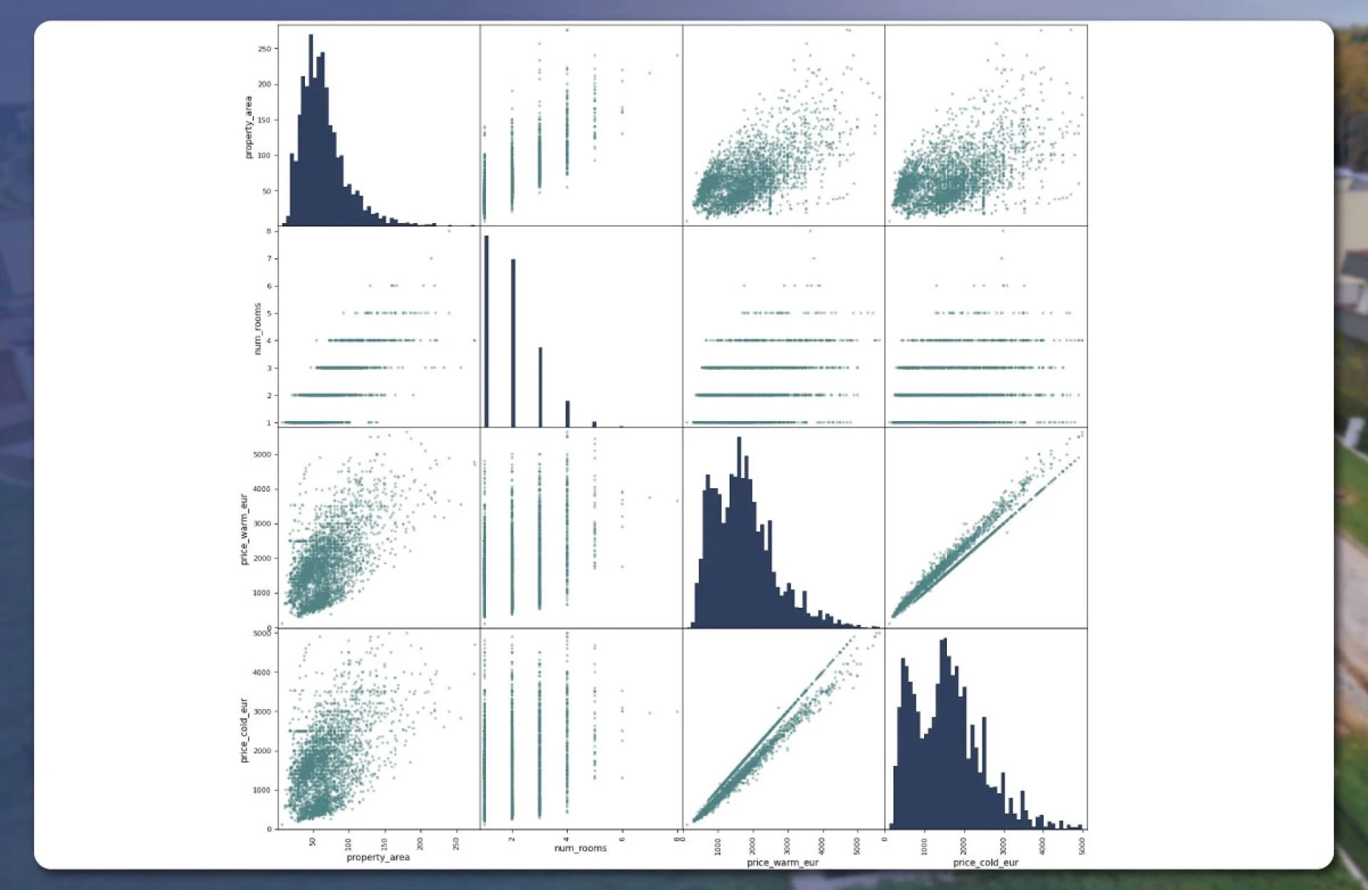
In the next step, we will make a scatter matrix for specific fields like several rooms, property areas, and prices. We will again use Panda for this

The data plotted on the histogram will appear like this.

For other visualization, we will use the Bokeh library for making beautiful and interactive graphs. First, we will import the necessary files.

Property Types

We collected data from 67 different cities in Germany, transferred them to a CSV file, and combined them all in a single data frame.

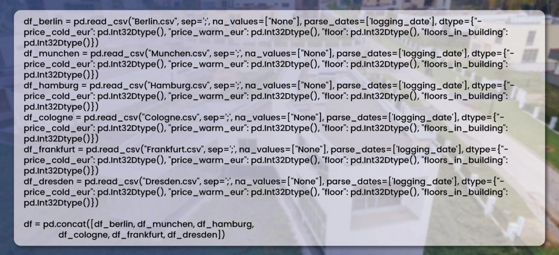
Now, we will find the property types distribution:

After replacing the ‘NA’ value with ‘unknown,’ we grouped the property types according to value and sorted the result by the amount. Then, to avoid the blue bars in Matplotlib style, we have specified the color palette. The final output will appear like these:

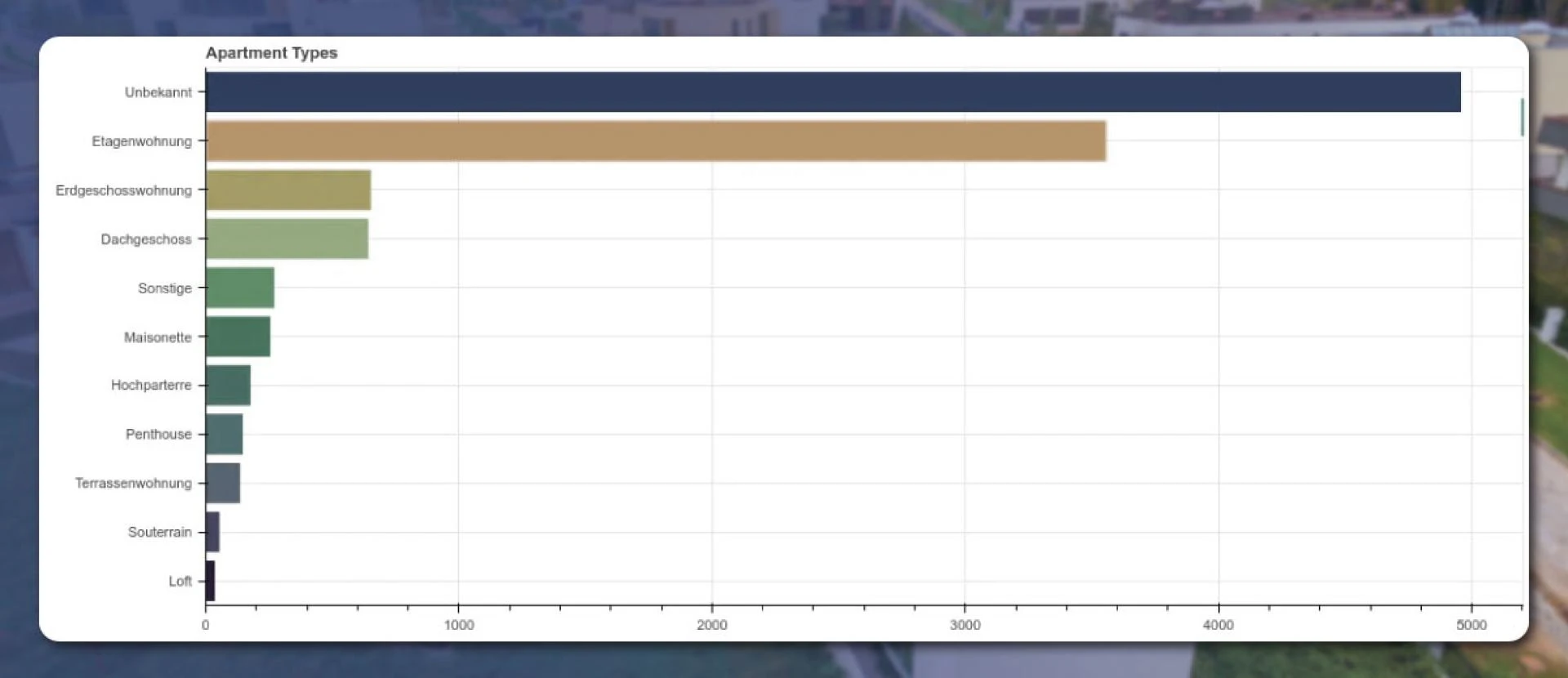
From the above image, several properties are without types. However, the apartment situated on the floor is the most popular one. The third and fourth types are under-the-roof and ground-floor apartments.

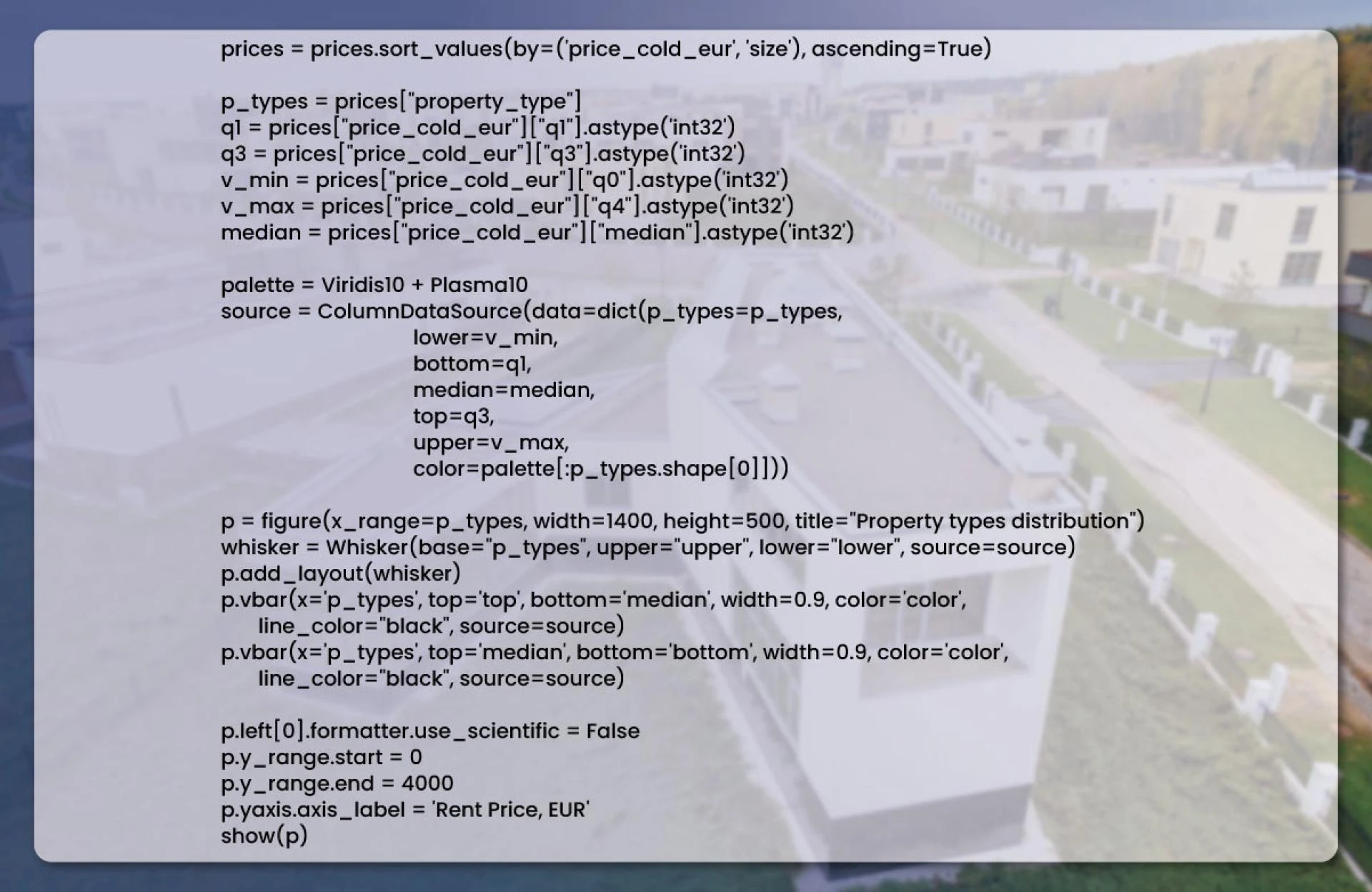
Now, let’s find the price distribution by type and combine the results in Pandas.

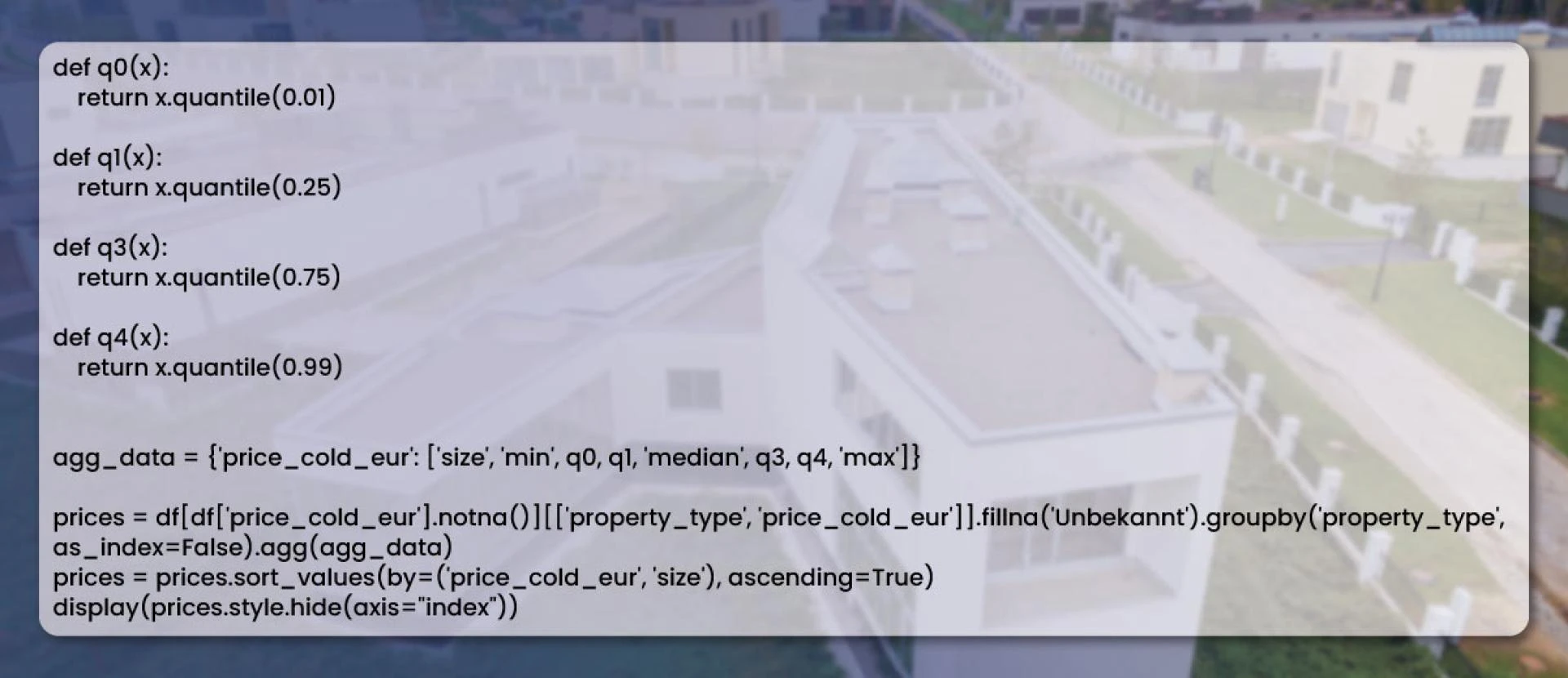
The results in the table form will appear like this:

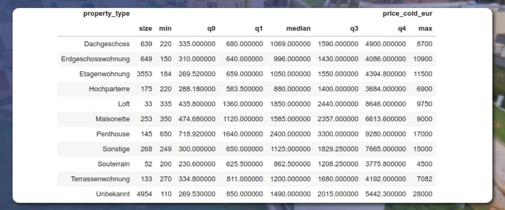
The box-and-whisker bplot gives the visual form of results like this:

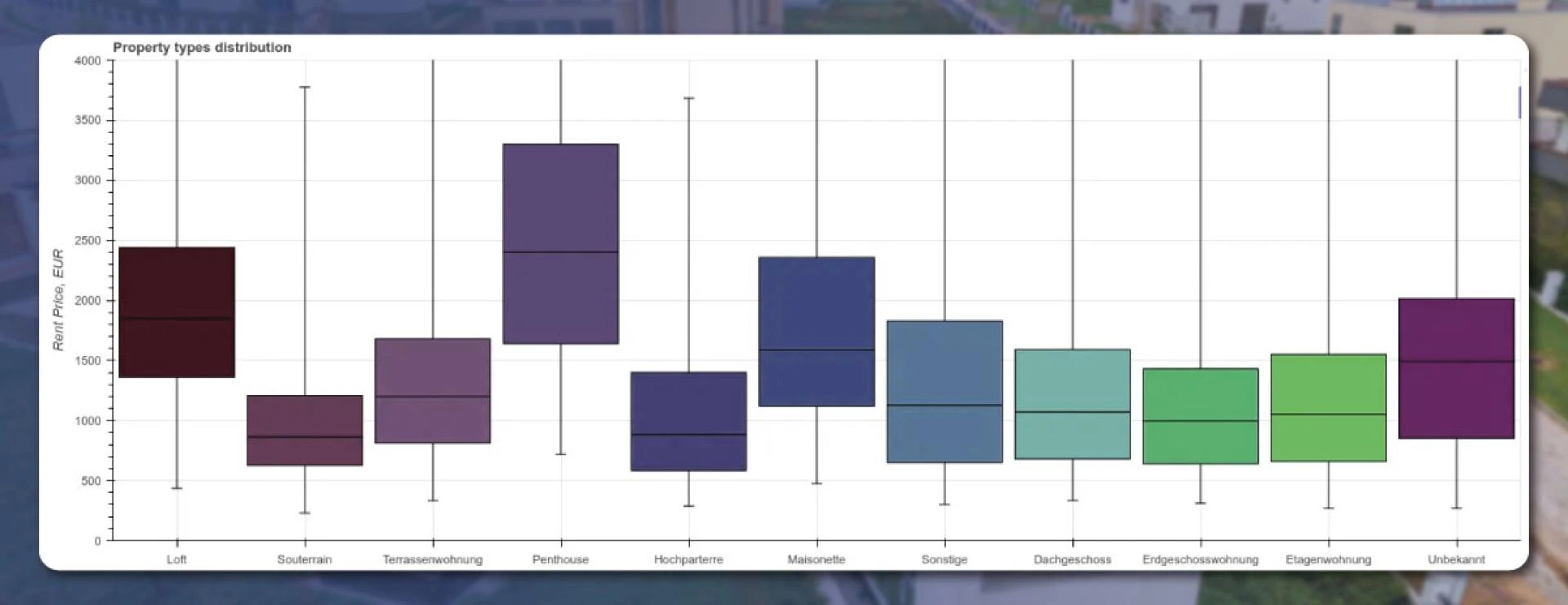
The penthouses are the most expensive, followed by standard apartments, under-the-roof, and ground-floor apartments.

Property Prices

Price Per Area

We obtain a scatter plot to understand the specific property size available for rent for a specific price. However, it requires only two arrays – X and Y. But, here, we will first create a list of property types and amounts

We will create three different arrays for the specific city. It includes the area in square meters, type, and price.

Here, I substituted the NULL property with ‘Unbekannt,’ which is not required for a scatter plot but for a graph. We will create a linear regression model and train using the data points. It will help in drawing a linear approximation:

We will draw the results:

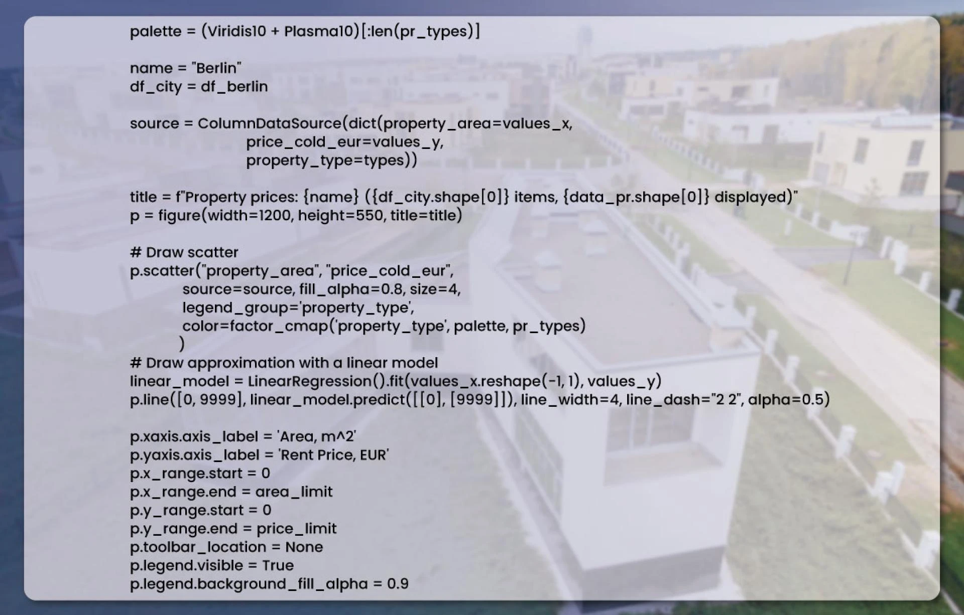
We will put the code in a separate get_figure_price_petr_area method to display different cities on the graph. Combining them in rows and columns, we will draw several Bokeh figures.

The plotted results will look like this:

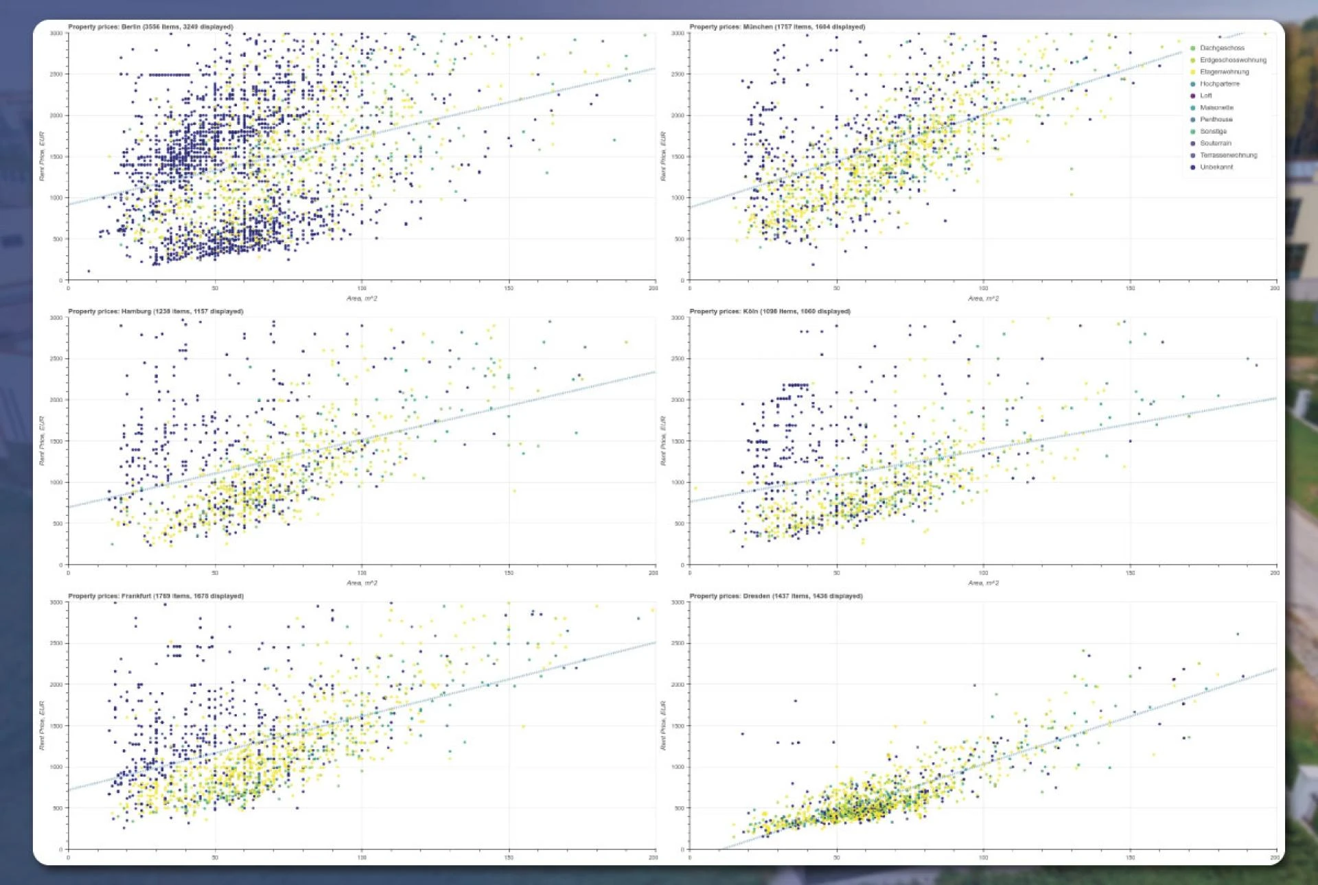
We will visually compare the number of properties available in the market.

Price and Area Histograms

Using a histogram, we will see the prices more compactly. The NumPy histogram method will perform all the calculations

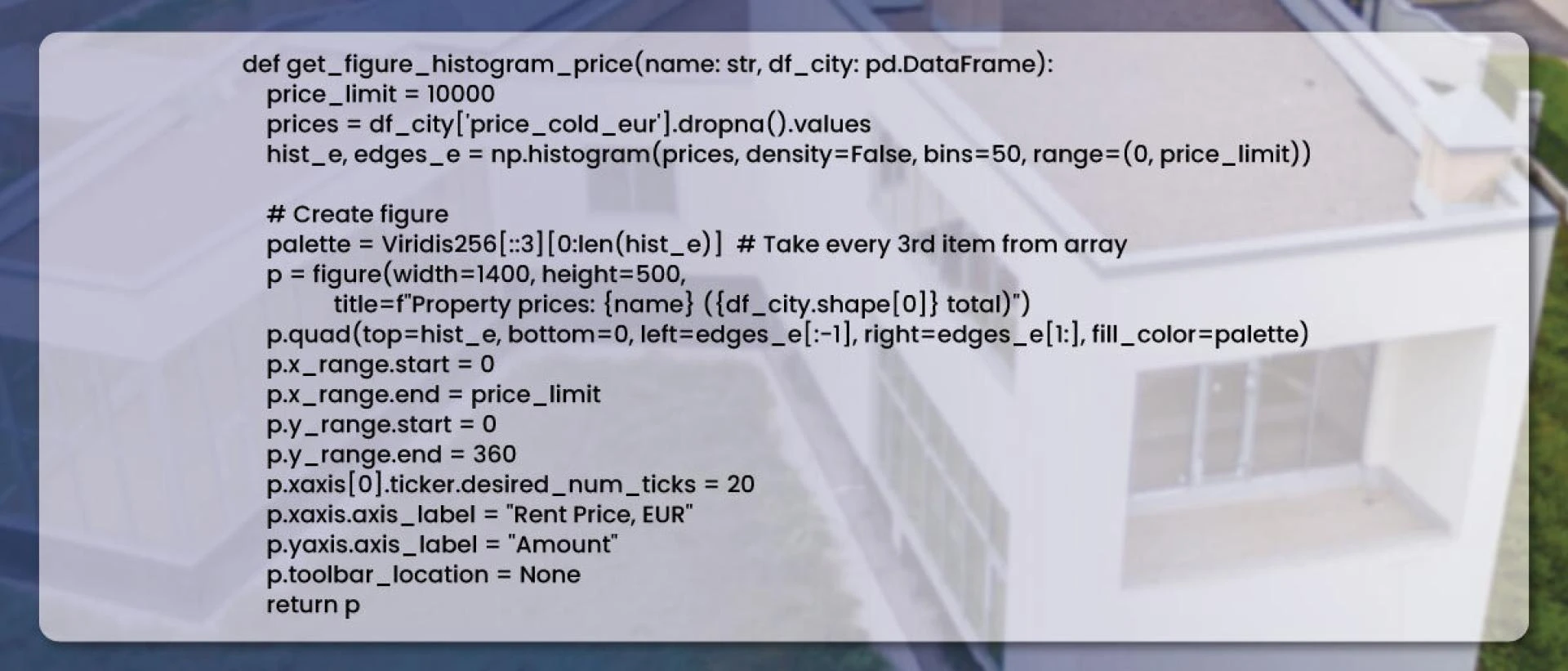
We used the same approach to draw the graph by mentioning several cities altogether:

The results correlate with the scatter plot.

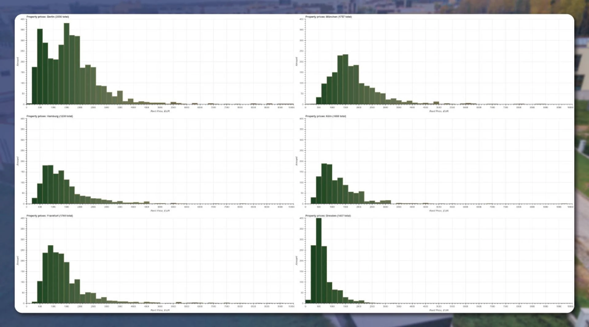
Munchen is the most expensive place, where the distribution peak is nearly €1,500, and has two peaks in Berlin. For the square-meter area, we will show the results only for Berlin

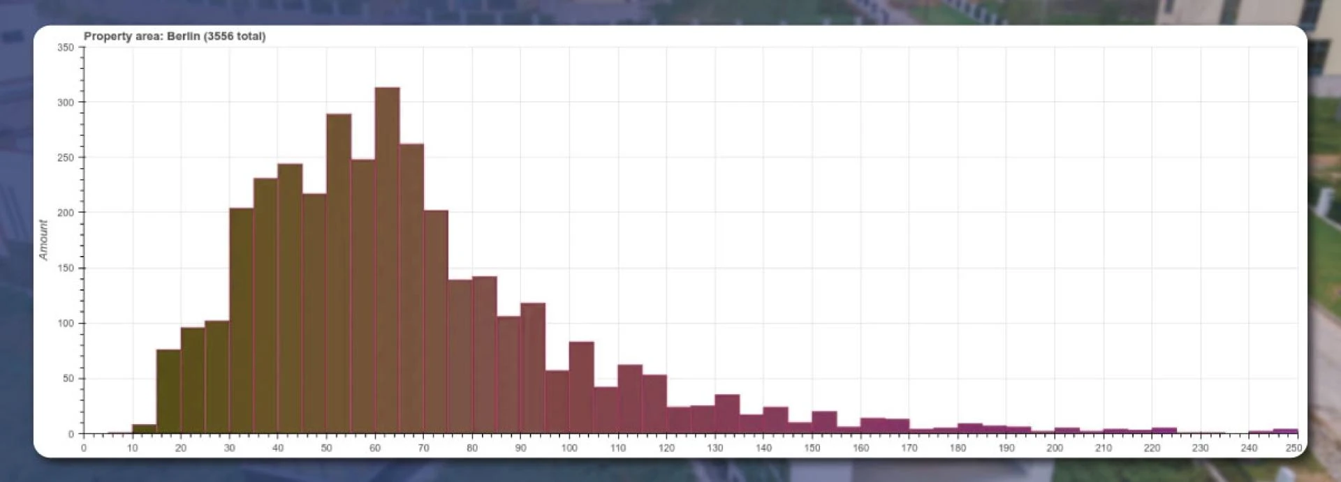
Several houses and apartments have an area of 30 to 70 square meters. Some properties are smaller than 10 square meters, while some are larger than 250 square meters.

Utility Costs

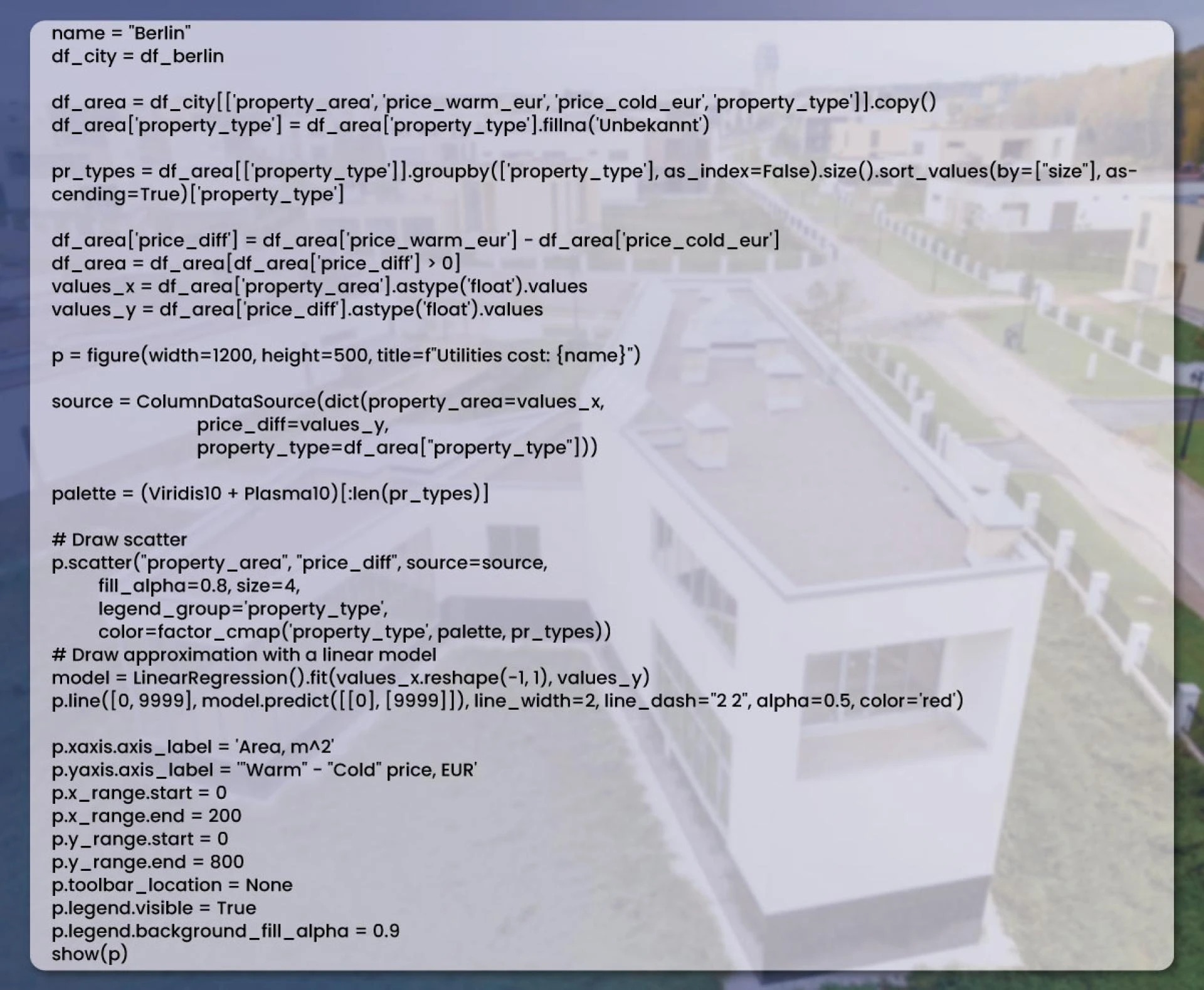
All apartments have two prices – warm and cold values. We will calculate the difference and design a scatter plot

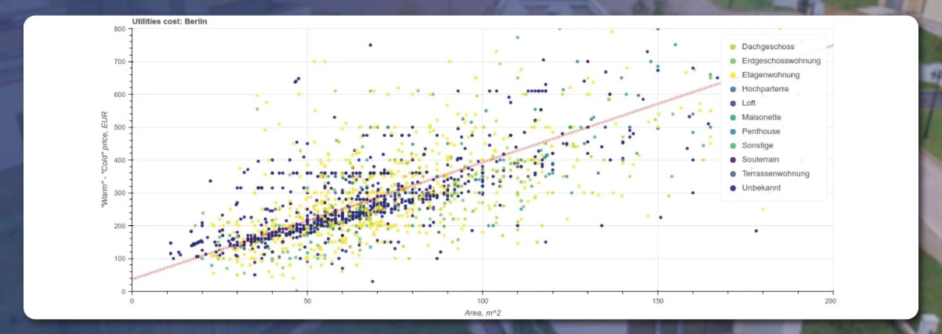
From the above image, we see that the results vary a lot. Different types of houses possess different insulation, heating, etc. The 50 square meter property has nearly 200 Euro utility costs per month. As the area doubles, the costs double.

Deposit

First, we will find out the type of data:

The results will appear like this:

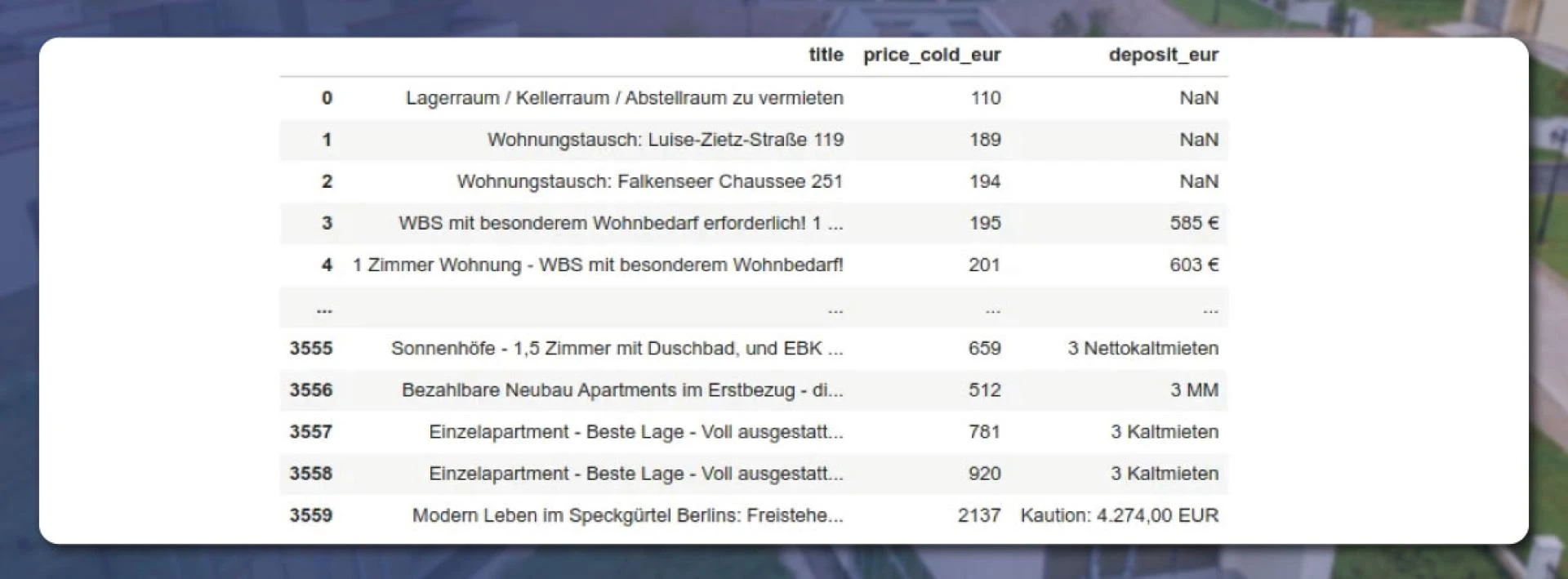
Displaying unique values is too easy. From the above image, we can see that values differ a lot. Some owners place the amount as a digit like ‘585 Euro’ while others use text metaphors like ‘3 MM’.

The output shows the text descriptions like ‘Drei Nettokaltmieten,’ ‘Zwei Monatsmiete, and so on. For parsing the values, we created two methods that transform a text string into numerical values.

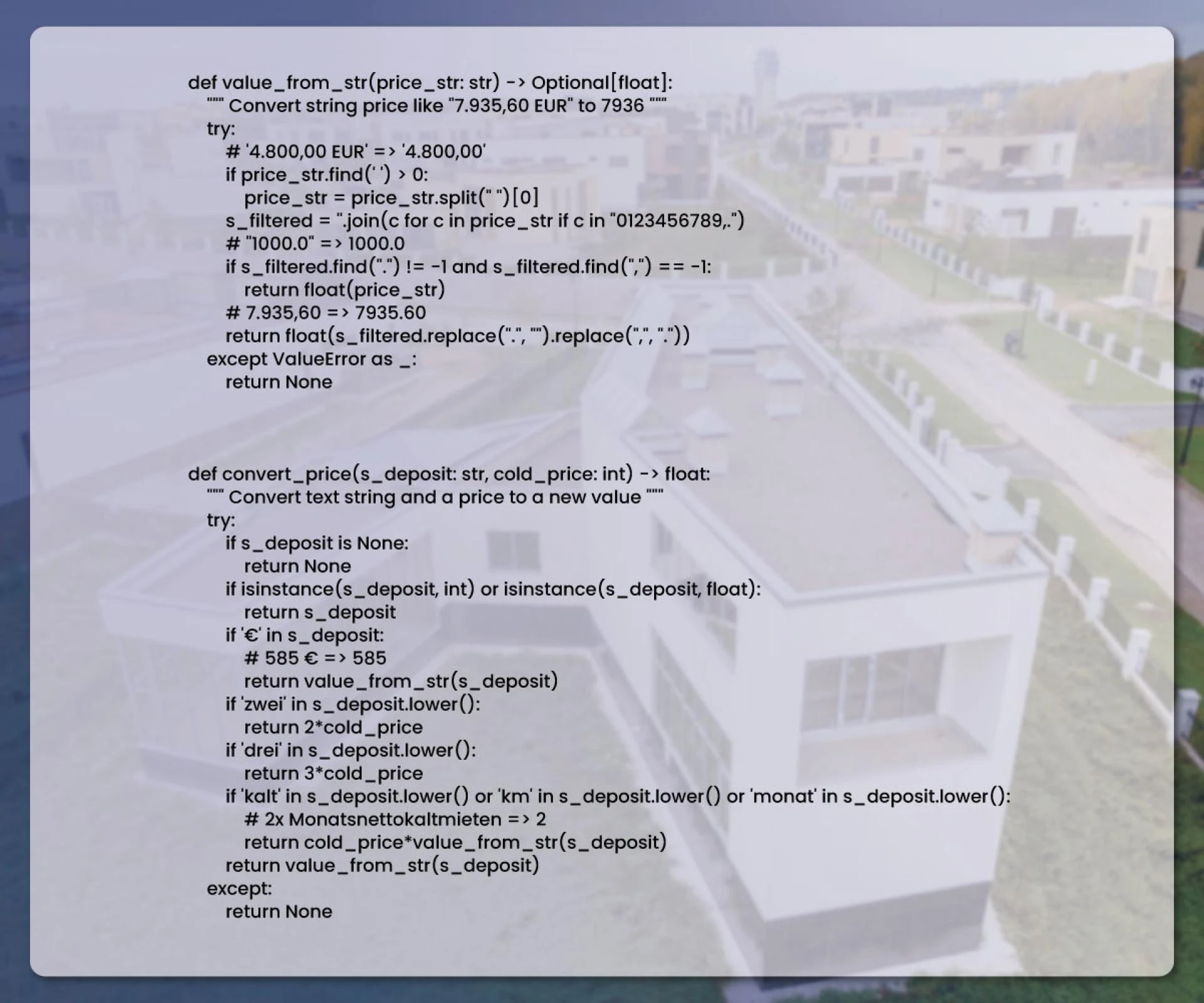
Using these methods, you can do the conversion like this:

Creating a column in the dataset with a deposit-to-price ratio is now easy.

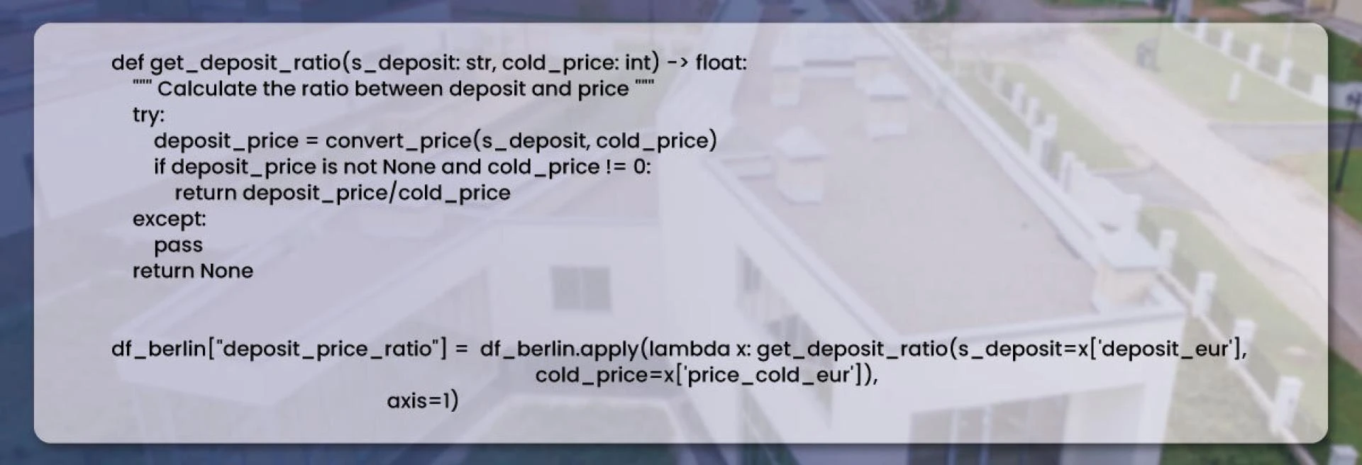
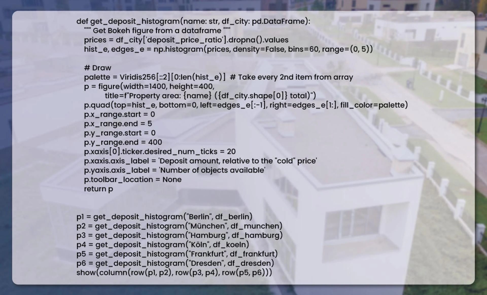
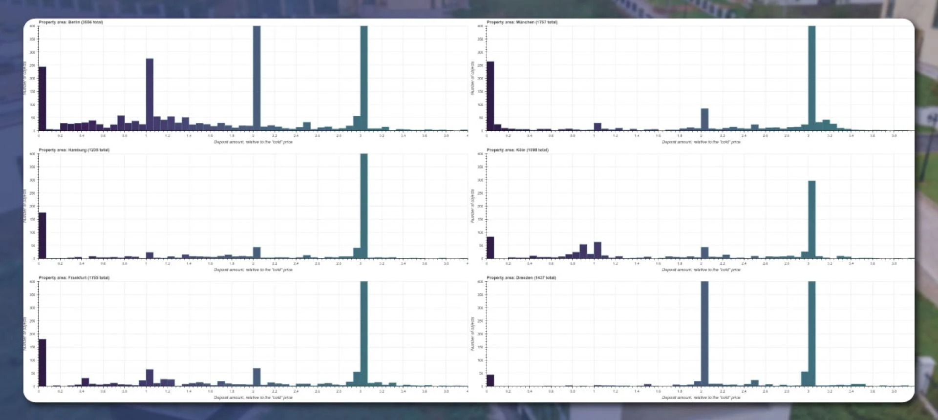
Using this new column, you can easily plot the histogram:

Property Owners

Numerous owners prefer to rent their properties alone, while others seek the agency’s help. To understand this, we will draw the distribution in the pie chart.

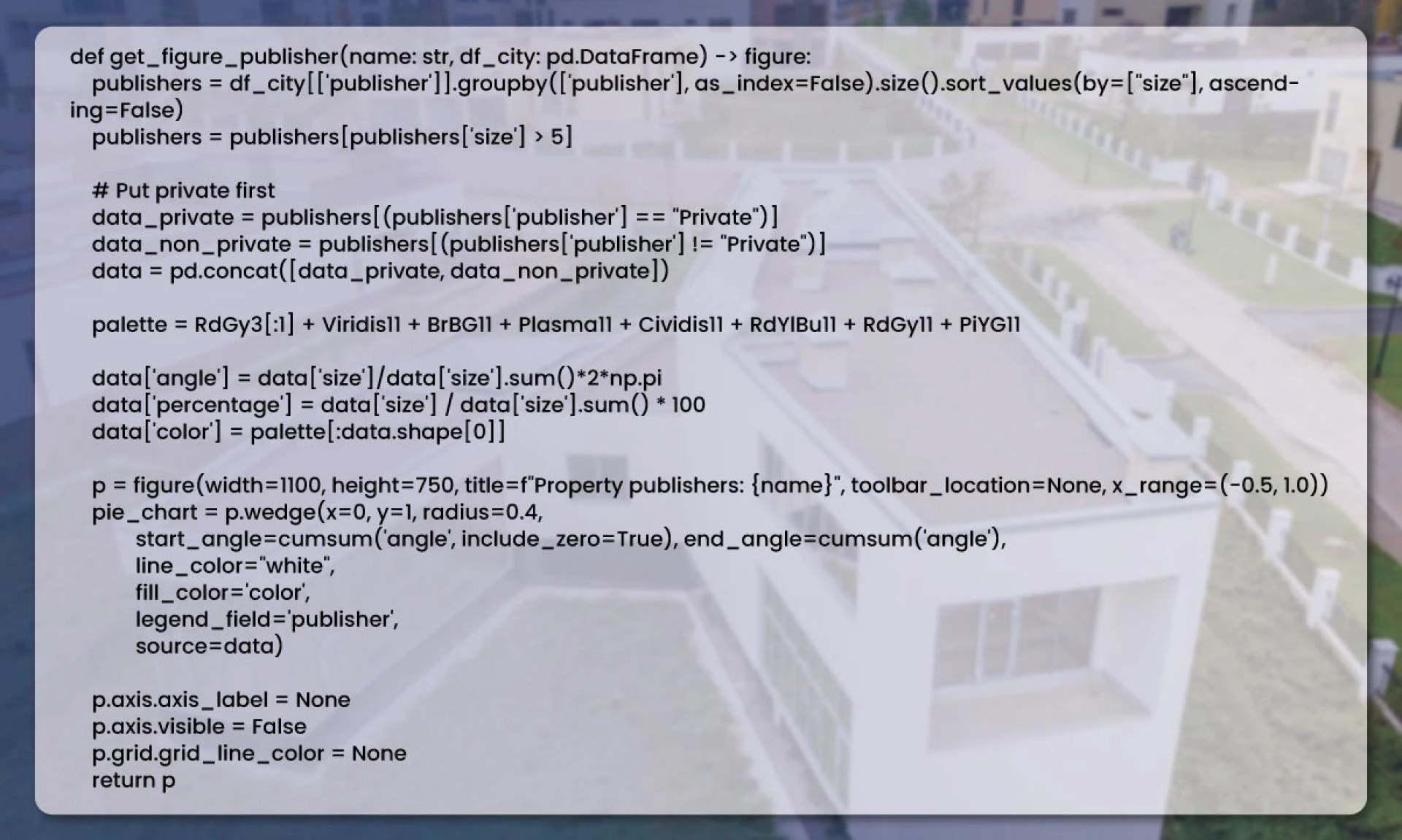
The publisher groups the data frame in the above code; results are available according to size. For groups, we use different colors.

The Berlin and Munchen cities results will appear like this:

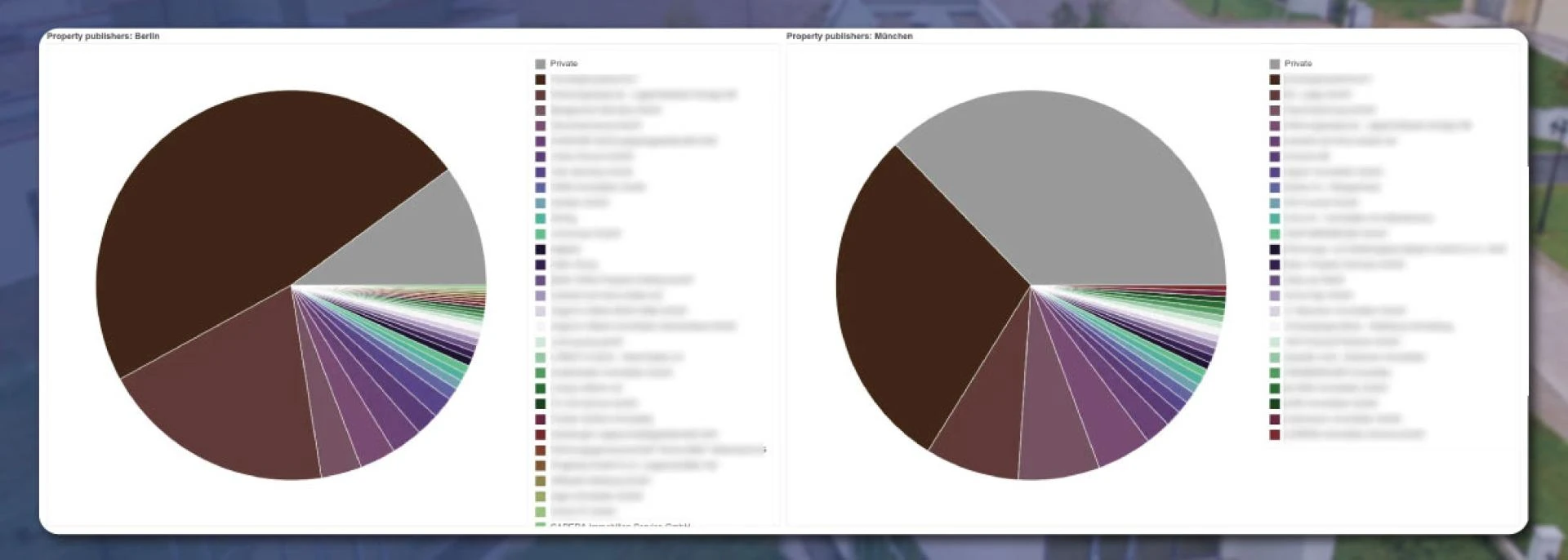
In Berlin, 8.5% of the real estate listing is by private individuals. In Munchen, it is 27%. A few agencies publish more than 50% of the properties.

Floor Numbers

Several houses and apartments do not have a specific floor number. Hence, we marked it as an ”unknown” value in such a case by implementing a custom key in Pandas. But, the challenging part is that while performing a Dataframe sort, the custome_key applies by Pandas not to a single value but to the ‘pd.Series’ object. Hence, we need a second method to update the values in the series.

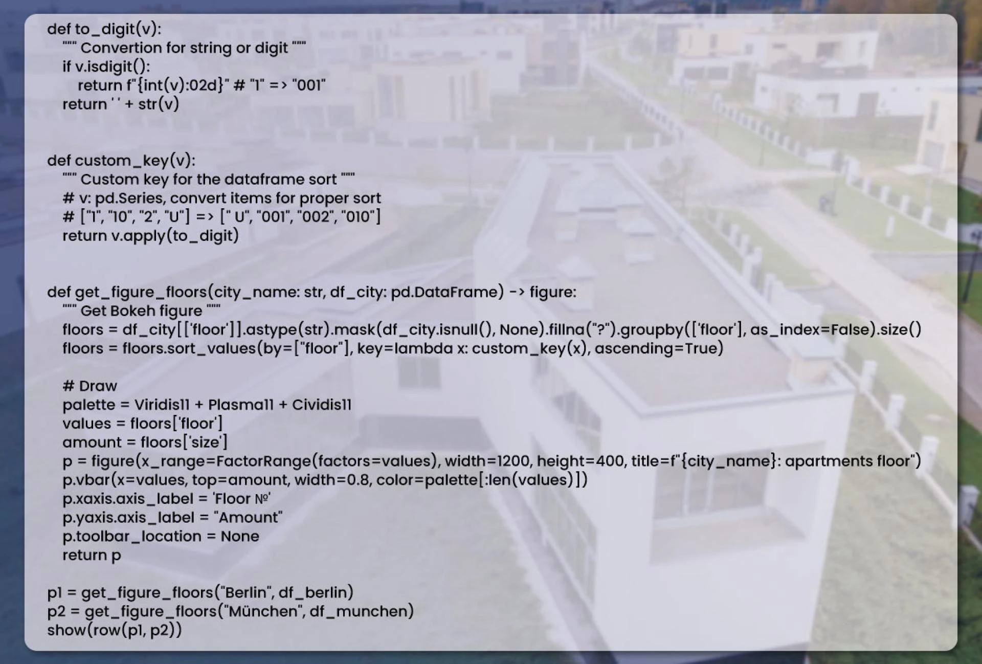
The results for Berlin and Munchen will appear like this:

We can see that most apartments in both cities lie on the 1st to 5th floors. But, several apartments have 10-20 floors. Exceptionally, an apartment in Berlin lies on the 87th floor.

Geo Visualization

We have to build a histogram before. Here, we will display estate objects on a geographic map. The two types of challenges that we may face are: Getting the coordinates and drawing the map.

Geocoding

We will again check our data. The data frame has different fields like addresses and regions. These fields are available for geocoding.

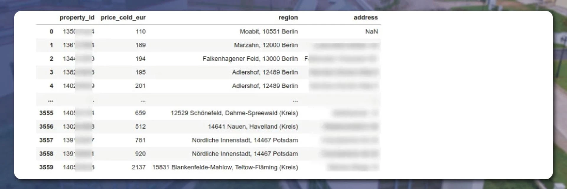
To find the coordinates, let’s use the GeoPy library.

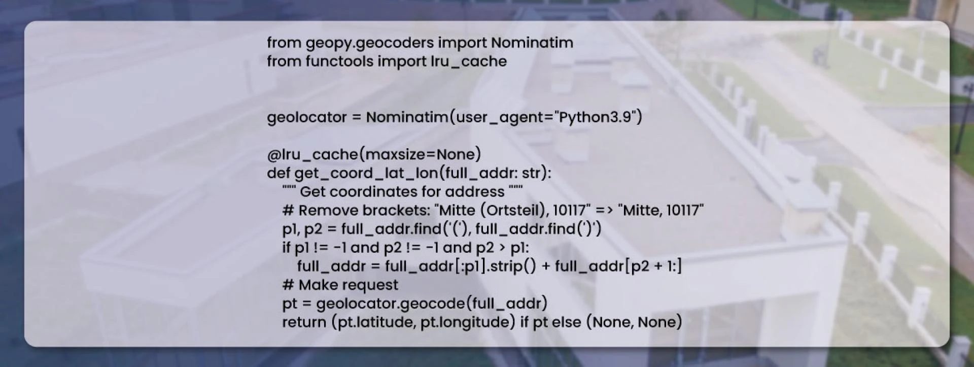
Although this was very simple, removing “(and)” brackets from the addresses was a significant challenge. Using the ‘Iru_cache’ method, it’s easy to request locations.

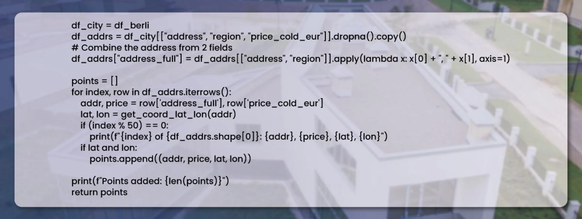
Map

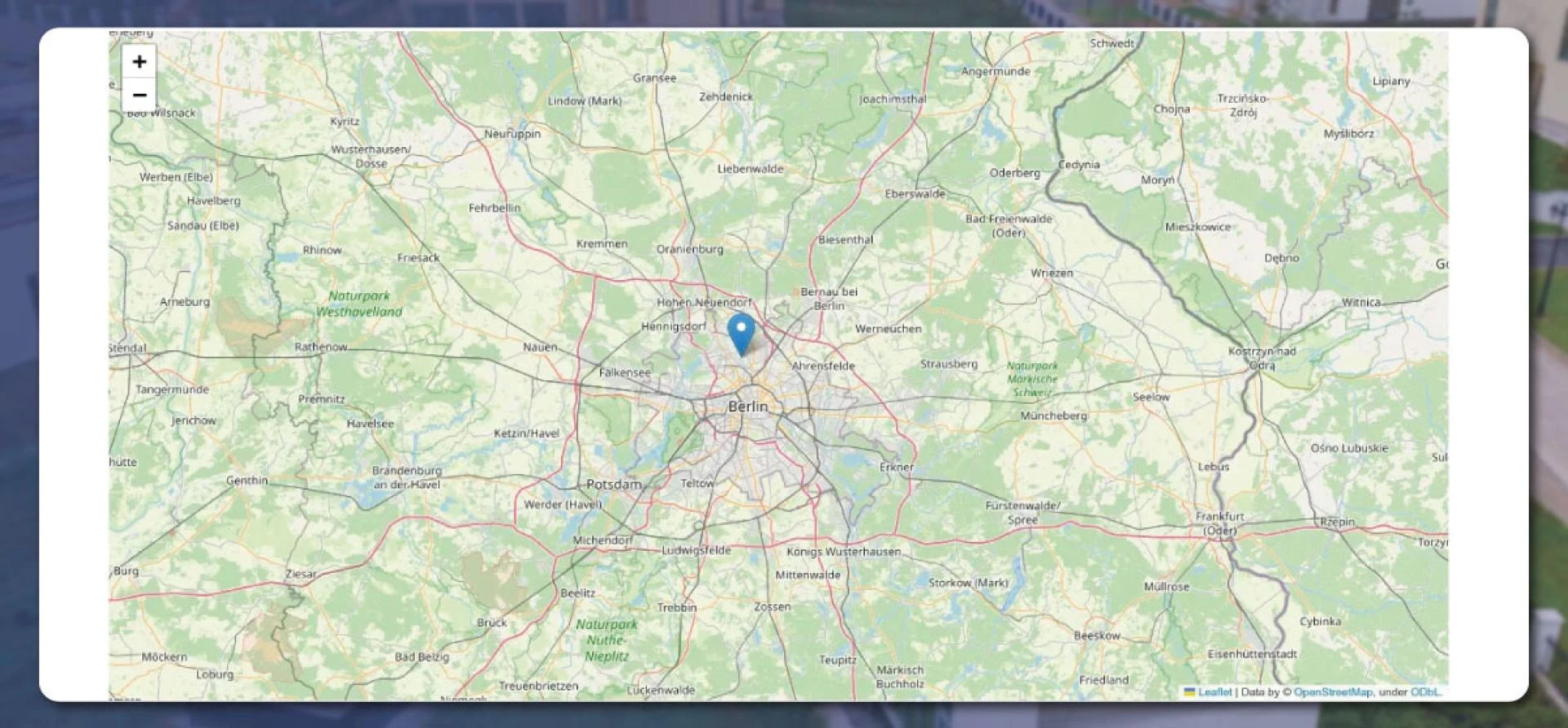
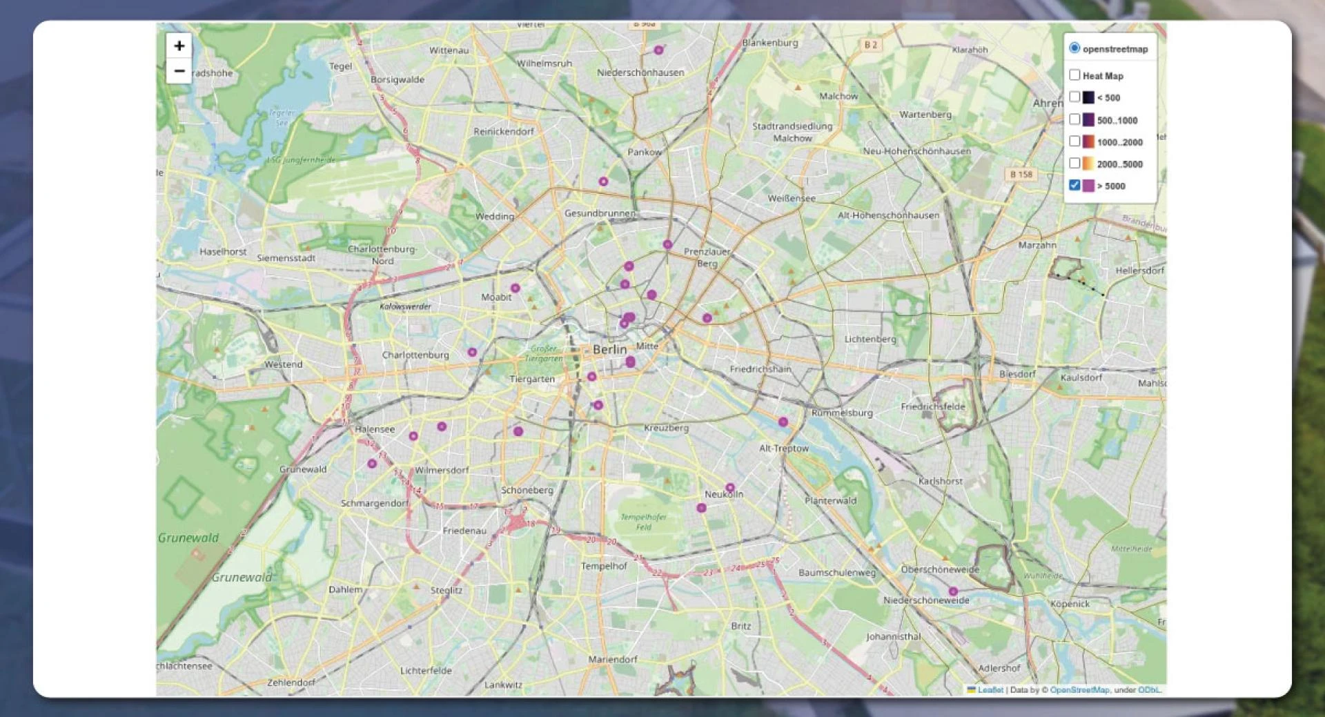
For drawing the map, we will use a free Folium library. The map having a mark will display several lines of code:

The code will give a clear, interactive map without any API code:

We will use Folium’sFolium’s Circle for each property and group the prices with the help of ”FeatureGroup.”

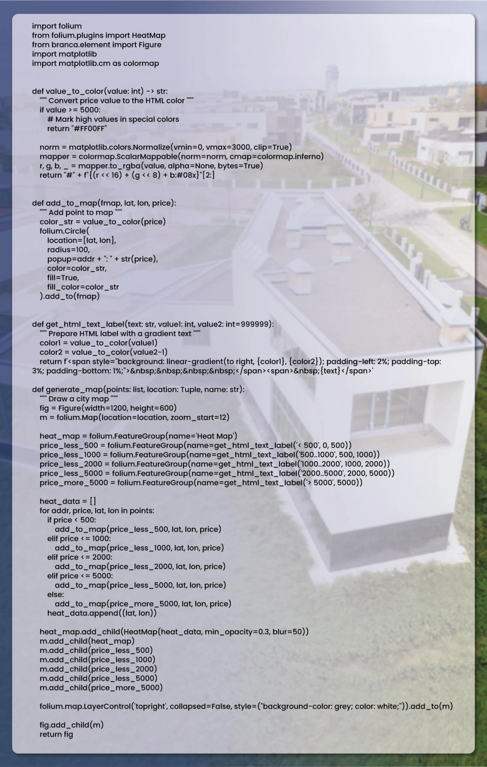
We have also used a heatmap to make the results look much better. The final results will appear like this:

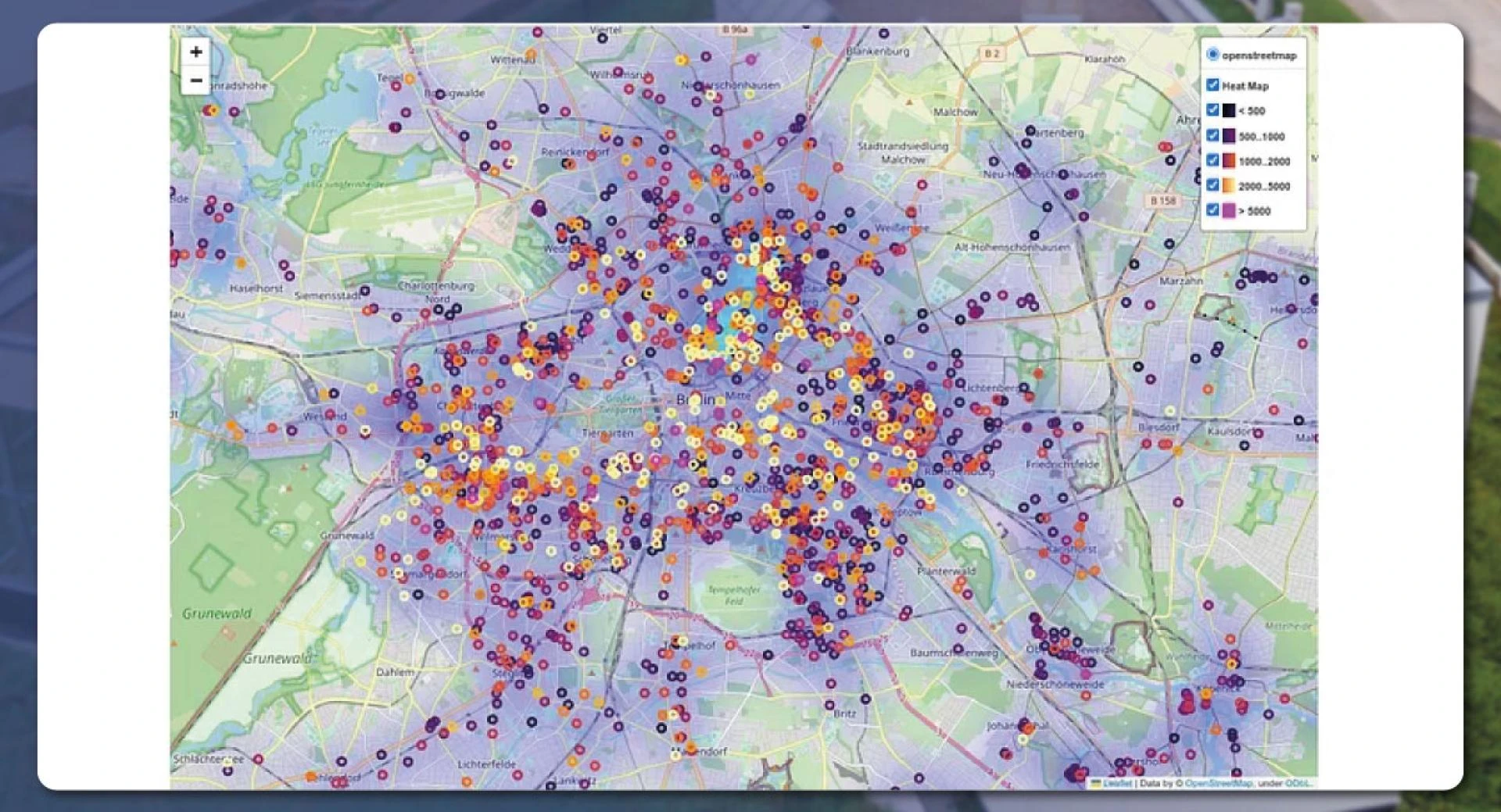
The real estate objects with more than 5000/m Euro are available evenly. The result is more or less automatic. In Berlin, areas surrounding the center are more expensive.

Rent Dynamics

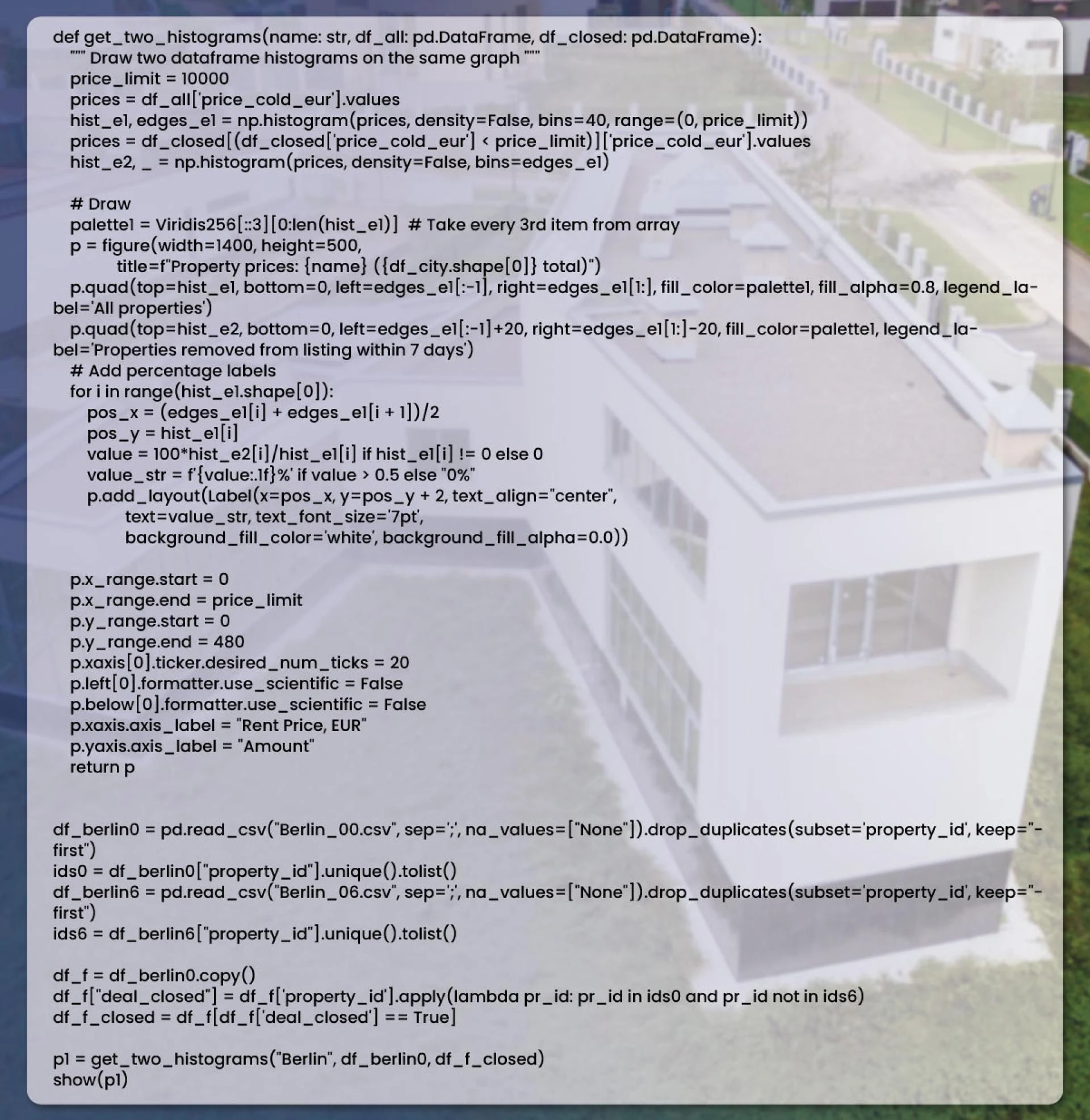
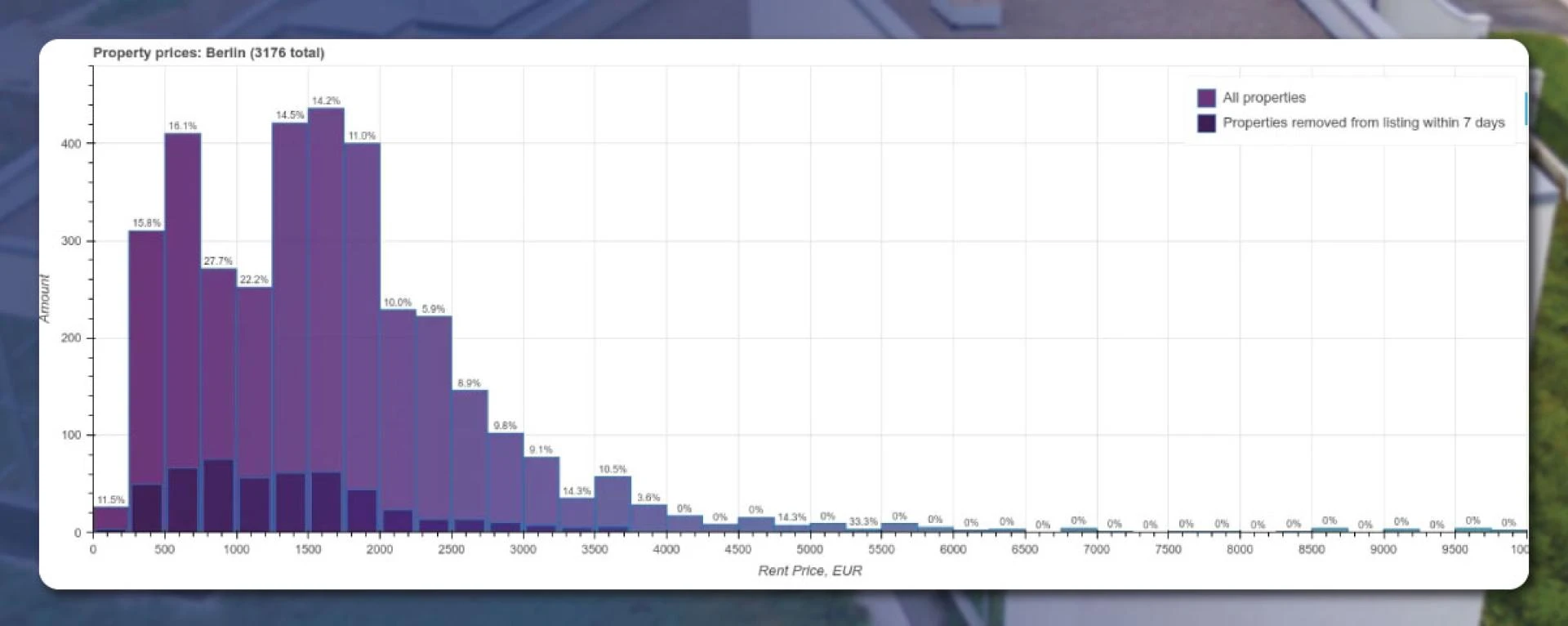
How quick is the renting process, and for how long it’s available for rent? This question is unpredictable. But, we will estimate the data by comparing the results of different days. Each property holds a different ID. We will save the data for the same city with an interval of 7 days and display two price histograms for all properties and the other for those removed within seven days.

To make the bars more readable, let’s add the percentage labels. The result will appear like this:

Anomalies Detection

In this step, we will find some anomalies – unusual and non-standard. For this, let’s use the Isolation Forest algorithm. We will use three features – Area, prices, and room numbers.

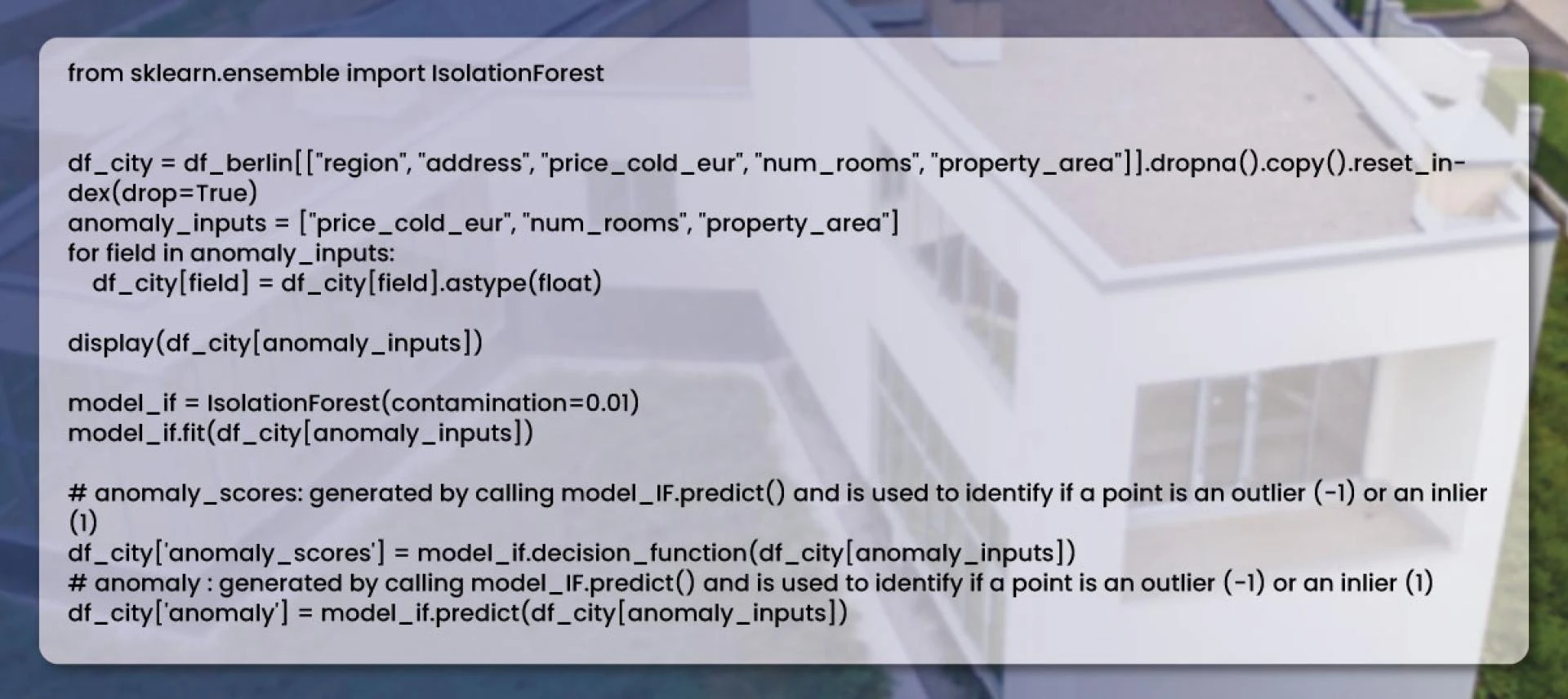
In the above code, the algorithm wants only one parameter. It is known as contamination. It determines the outlier’s proportion. Let’s set it to 1%. We get the result after using the ‘fit’ method. The ‘decision_function’ returns the anomaly score. The ‘predict’ method returns +1 if the object is an inlier and -1 If it is an outlier

The result is:

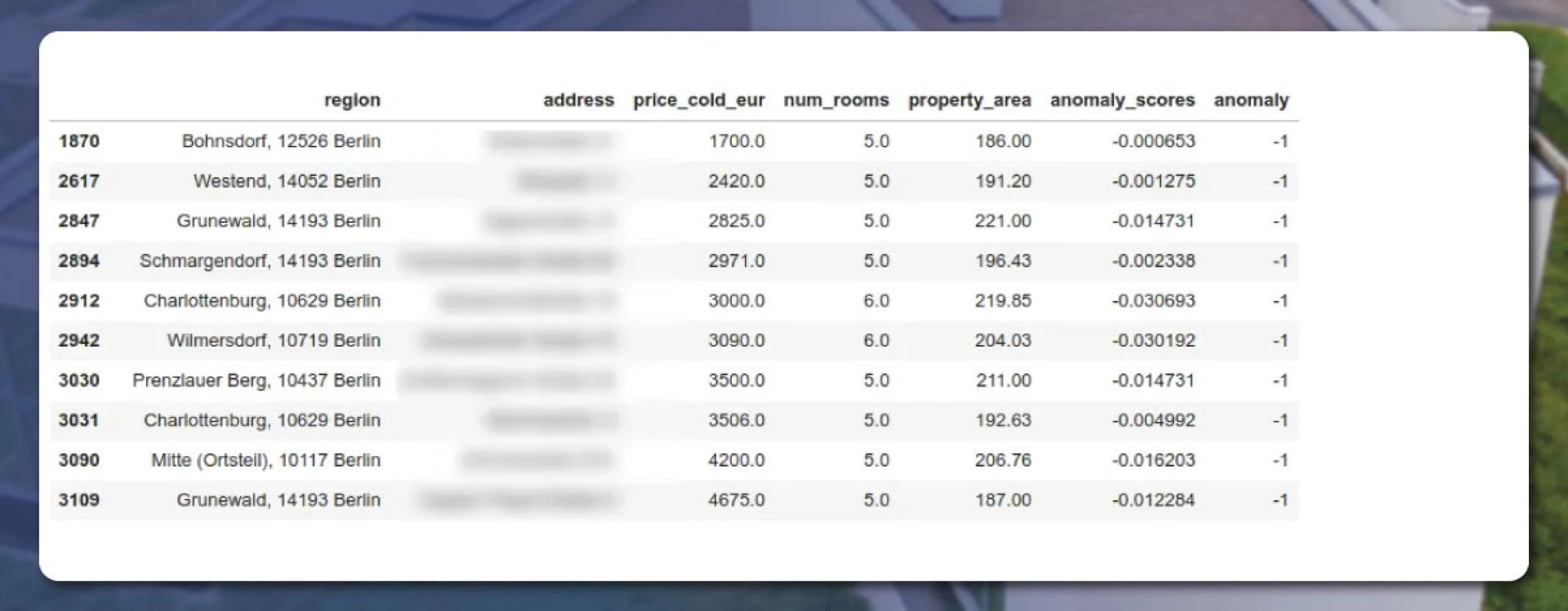
To explain the results graphically, let’s seek the help of the SHAP Python package.

Let’s examine the property within the number 3030.

We found that the prices were acceptable. But, the algorithm treated the 211 square meter property area and the number of 5 rooms as unusual. By displaying a scatter plot, let’s check how the algorithm works. Let’s see how the number of rooms and price impact the Shapley values.

The result will appear like this:

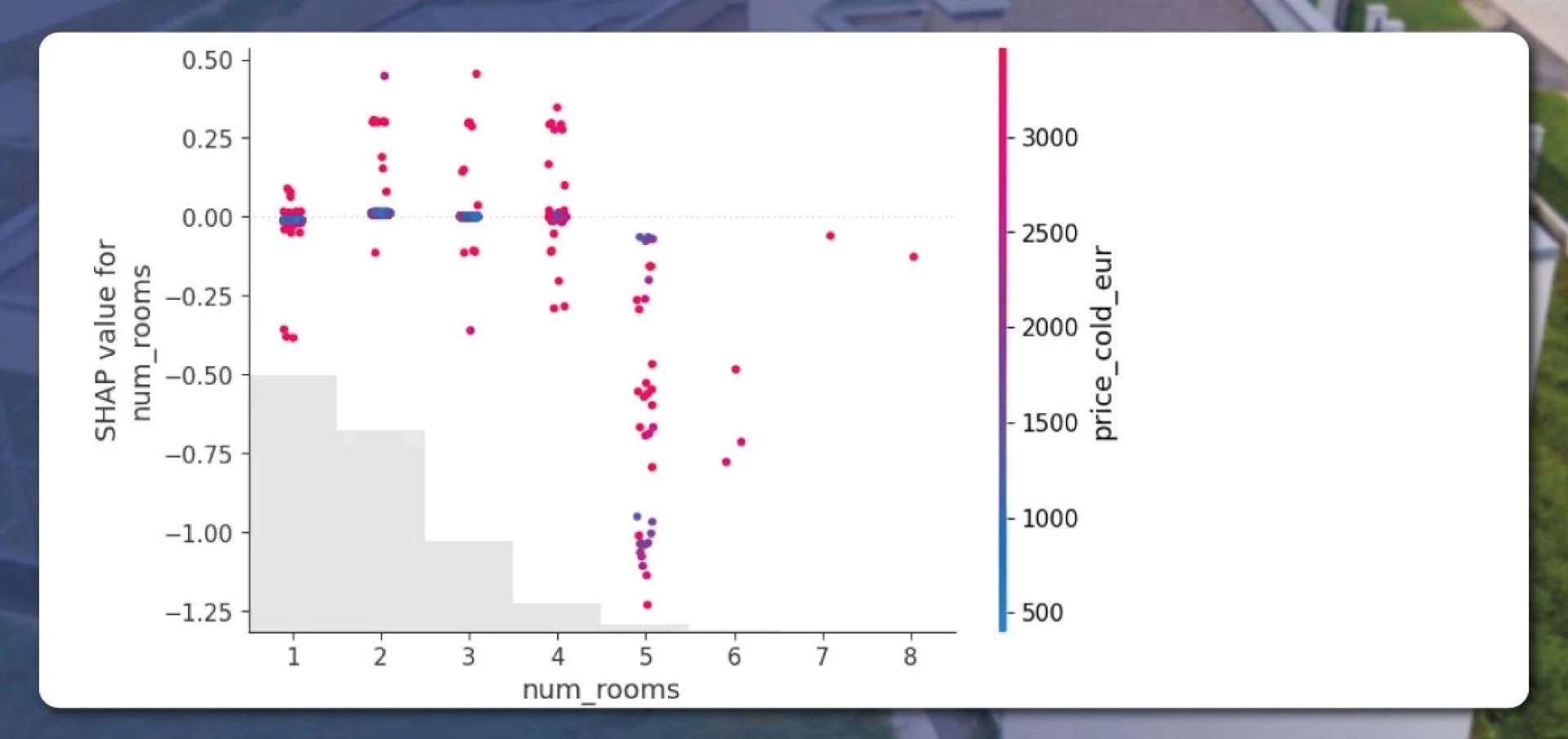
Here, we can see that number of rooms above 4 affects the score the most.

Word Cloud

Here, we will find which word is trendy in the estate titles:

Using a Python WordCloud library, we will do this in several lines of code:

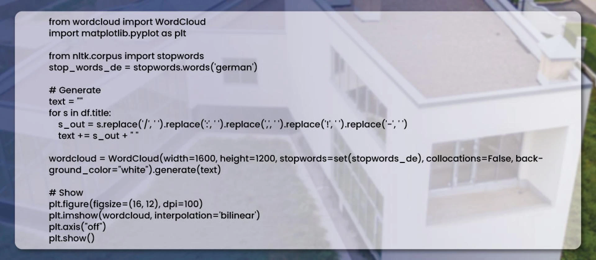
The result will appear like this:

Certain words like apartment, room, bright, modern, beautiful, and balcony are famous words we see.

For more information, get in touch with Actowiz Solutions now! You can also reach us for all your web scraping service and mobile app data scraping service requirements.